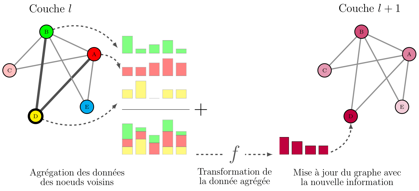
Message Passing

Scheme of message passing

\documentclass[border=3pt,tikz]{standalone}
\usepackage[dvipsnames]{xcolor}
\usepackage{pgfplots}
\definecolor{taupegray}{rgb}{0.55, 0.52, 0.54}
\def\general_height{0.2}

\usepackage{tikz-network}

\begin{document}
\begin{tikzpicture}

\Text[x=-0.18,y=3cm]{\Large Couche $l$}
\Text[x=14cm,y=3cm]{\Large Couche $l+1$}

\begin{scope}[scale=2]
\Vertex[x=0.88,y=0.48,label=A,color=red]{A}
\Vertex[x=-0.18,y=0.98,label=B,color=green]{B}
\Vertex[x=-1,y=0.12,label=C,color=pink]{C}
\Vertex[x=-0.42,y=-0.9,label=D,color=yellow,style={line width=1mm}]{D}
\Vertex[x=0.72,y=-0.69,label=E,color=cyan]{E}
\Edge[color=gray](A)(B)
\Edge[color=gray](A)(C)
\Edge[lw=3](A)(D)
\Edge[color=gray](A)(E)
\Edge[color=gray](B)(C)
\Edge[lw=3](B)(D)
\Edge[color=gray](B)(E)
\end{scope}

\begin{scope}[xshift=3cm]
\Vertex[x=0,y=0,Pseudo]{K}
\begin{axis}[ybar stacked,
height=\general_height\textwidth,
 bar width=13pt,ymin=0,
 x=17pt,
 ytick=\empty,
 xtick=\empty,
 hide axis]
    \addplot[fill=red,opacity=0.5] coordinates
        {(0,0.1) (1,0.1) (2,0.15) (3,0.2) (4,0.15)};
    \end{axis}

\Vertex[x=0,y=1,Pseudo]{L}
\begin{axis}[ybar stacked, 
yshift = 1cm,
height=\general_height\textwidth,
 bar width=13pt,ymin=0,
 x=17pt,
 ytick=\empty,
 xtick=\empty,
 hide axis]
    \addplot[fill=green,opacity=0.5] coordinates
        {(0,0.2) (1,0.05) (2,0.1) (3,0.15) (4,0.05)};
    \end{axis}

\Vertex[x=0,y=-1,Pseudo]{M}
\begin{axis}[ybar stacked, 
yshift = -1cm,
height=\general_height\textwidth,
 bar width=13pt,ymin=0,
 x=17pt,
 ytick=\empty,
 xtick=\empty,
 hide axis]
    \addplot[fill=yellow,opacity=0.5] coordinates
        {(0,0.1) (1,0.2) (2,0) (3,0.1) (4,0.1)};
    \end{axis}

\draw (0,-1.5cm) -- (3,-1.5cm);
 \Text[x=3.5,y=-1.5cm]{\Huge $\mathbf{+}$}

\begin{axis}[ybar stacked,
height=0.27\textwidth,
yshift = -3.5cm,
 bar width=13pt,ymin=0,
 x=17pt,
 ytick=\empty,
 xtick=\empty,
 hide axis]
 \addplot[fill=yellow,opacity=0.5] coordinates
        {(0,0.1) (1,0.2) (2,0) (3,0.1) (4,0.1)};
  \addplot[fill=red,opacity=0.5] coordinates
        {(0,0.1) (1,0.1) (2,0.15) (3,0.2) (4,0.15)};
 \addplot[fill=green,opacity=0.5] coordinates
        {(0,0.2) (1,0.05) (2,0.1) (3,0.15) (4,0.05)};   
 \end{axis}
 \Vertex[x=3,y=-3.5,Pseudo]{N}  
\end{scope}
\node[align=center,text width=5cm] at (1,-4.5) {\large Agrégation des données des noeuds voisins};

\Edge[bend=35,style={dashed},Direct](A)(K)
\Edge[bend=35,style={dashed},Direct](B)(L)
\Edge[bend=-35,style={dashed},Direct](D)(M)

\begin{scope}[xshift=10cm,yshift=-3.5cm]
    \begin{axis}[ybar stacked, 
height=\general_height\textwidth,
 bar width=13pt,ymin=0,
 x=17pt,
 ytick=\empty,
 xtick=\empty,
 hide axis]
    \addplot[fill=purple] coordinates
        {(0,0.2) (1,0.15) (2,0.1) (3,0.1) };
    \end{axis}
 \Vertex[x=0,y=0,Pseudo]{N'}    
\Vertex[x=2,y=0,Pseudo]{N''}    


\end{scope}

\Edge[style={dashed},Direct,label={\Huge $f$}](N)(N')
\node[align=center,text width=3.5cm] at (8cm,-4.5) {\large Transformation de la donnée agrégée};


\begin{scope}[xshift=14cm,scale=2]
    \Vertex[x=0.88,y=0.48,label=A,color=purple,opacity=0.5]{A2}
\Vertex[x=-0.18,y=0.98,label=B,color=purple,opacity=0.7]{B2}
\Vertex[x=-1,y=0.12,label=C,color=purple,opacity=0.4]{C2}
\Vertex[x=-0.42,y=-0.9,label=D,color=purple]{D2}
\Vertex[x=0.72,y=-0.69,label=E,color=purple,opacity=0.2]{E2}
\Edge[color=gray](A2)(B2)
\Edge[color=gray](A2)(C2)
\Edge[color=gray](A2)(D2)
\Edge[color=gray](A2)(E2)
\Edge[color=gray](B2)(C2)
\Edge[color=gray](B2)(D2)
\Edge[color=gray](B2)(E2)
\end{scope}
\node[align=center,text width=5.5cm] at (13cm,-4.5) {\large Mise à jour du graphe avec la nouvelle information};

\Edge[bend=-35,style={dashed},Direct](N'')(D2)


\end{tikzpicture}
\end{document}