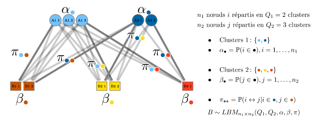
Latent block model
Probabilistic model for bipartite networks, credits to Louis Lacoste
\documentclass[border=3pt,tikz]{standalone}
\usepackage{pgfplots}
\usepackage[dvipsnames,table,xcdraw]{xcolor}
\usepackage{tikz}
\usepackage{amsmath}
\usepackage{amssymb}
\usepackage{enumitem}
\usepackage[outline]{contour} % glow around text
\contourlength{0.4pt}
\definecolor{electricblue}{rgb}{0.49, 0.98, 1.0}
\definecolor{cyanind}{rgb}{0.0, 0.4, 0.65}
\definecolor{blueind}{rgb}{0.45, 0.76, 0.98}
\definecolor{burntorange}{rgb}{0.8, 0.33, 0.0}
\definecolor{goldenyellow}{rgb}{1.0, 0.87, 0.0}
\definecolor{peach}{rgb}{1.0, 0.23, 0.13 }

\usetikzlibrary{arrows,automata}

\begin{document}
\begin{tikzpicture}[scale=0.35]
    \tikzstyle{every state}=[draw, text=black,scale=0.95,
    transform shape]
    \tikzstyle{every state}=[draw=none,text=black,scale=0.75,
    transform shape]
    \tikzset{edge_proba/.style={draw=white, fill=none,
                text=black}}

    \tikzstyle{every node}=[fill=blueind]
    \node[edge_proba] (pi1) at (1,5.7)
    {\textbf{$\alpha_{{\color{blueind}\bullet}}$}};
    \node[state, draw=black!50] (R11) at (0,5) {\textbf{A1 1}};
    \node[state, draw=black!50] (R12) at (1,5) {\textbf{A1 2}};
    \node[state, draw=black!50] (R13) at (2,5) {\textbf{A1 3}};

    \tikzstyle{every node}=[fill=cyanind]
    \node[edge_proba] (pi2) at (6.75,5.7)
    {\textbf{$\alpha_{{\color{cyanind}\bullet}}$}};
    \node[state, draw=black!50] (R21) at (6.25,5)
    {\textbf{A2 1}};
    \node[state, draw=black!50] (R22) at (7.25,5)
    {\textbf{A2 2}};

   % \tikzstyle{every node}=[fill=electricblue]
    %\node[edge_proba] (pi3) at (10,5.7)
    %{\textbf{$\alpha_{{\color{electricblue}\bullet}}$}};
    %\node[state, draw=black!50] (R31) at (10,5) {\textbf{R31}};

    \tikzstyle{every node}=[fill=burntorange, shape=rectangle]
    \node[edge_proba] (pi3) at (-2.5,-1)
    {\textbf{$\beta_{{\color{burntorange}\bullet}}$}};
    \tikzstyle{every state}=[draw=none,text=black,scale=0.75,
    transform shape, shape=rectangle]
    \node[state, draw=black!50] (C11) at (-3,0) {\textbf{B1 1}};
    \node[state, draw=black!50] (C12) at (-2,0) {\textbf{B1 2}};
    \tikzstyle{every node}=[fill=goldenyellow, shape=rectangle]
    \node[edge_proba] (pi3) at (4,-1)
    {\textbf{$\beta_{{\color{goldenyellow}\bullet}}$}};
    \node[state, draw=black!50] (C21) at (3.5,0) {\textbf{B2 1}};
    \node[state, draw=black!50] (C22) at (4.5,0) {\textbf{B2 2}};
    \tikzstyle{every node}=[fill=peach, shape=rectangle]
    \node[edge_proba] (pi3) at (10,-1)
    {\textbf{$\beta_{{\color{peach}\bullet}}$}};
    \node[state, draw=black!50] (C31) at (10,0) {\textbf{B3 1}};

    \tikzstyle{every edge}=[-,>=stealth',shorten
    >=1pt,auto,draw,line width=1.5pt,draw opacity=0.2]

    \path (R11) edge[-,>=stealth',shorten
            >=1pt,auto,draw=gray,line width=1.5pt, fill=gray, opacity=1] node[midway, left,
            fill=none] {\contour{white}{$\pi_{{\color{blueind}\bullet}{\color{burntorange}\bullet}}$}}
    (C11);
    \path (R11) edge (C12);
    \path (R11) edge  (C21);
    \path (R11) edge  (C22);

    \path (R11) edge  (C31);
    \path (R12) edge  (C31);
    \path (R13) edge  [-,>=stealth',shorten
    >=1pt,auto,draw=gray,line width=1.5pt, fill=gray, opacity=1] node[pos = 0.75, right = -0.6cm,
    fill=none] {\contour{white}{$\pi_{{\color{blueind}\bullet}{\color{peach}\bullet}}$}}(C31) ;


    \path (R12) edge  (C11);
    \path (R12) edge  (C12);
    \path (R12) edge  (C21);
    \path (R12) edge  (C22);

    \path (R13) edge [] (C11);
    \path (R13) edge  (C12);
    \path (R13) edge  (C21);
    \path (R13) edge[-,>=stealth',shorten
            >=1pt,auto,draw=gray,line width=1.5pt, fill=gray, opacity=1] node[pos=0.7, right = -0.6cm,
            fill=none] {\contour{white}{$\pi_{{\color{blueind}\bullet}{\color{goldenyellow}\bullet}}$}}
    (C22);


    \path (R21) edge  (C22);
    \path (R21) edge  (C31);

    \path (R22) edge  (C21);
    \path (R22) edge  (C22);
    \path (R21) edge[-,>=stealth',shorten
            >=1pt,auto,draw=gray,line width=1.5pt, fill=gray, opacity=1] node[pos=0.2,
            right = -0.2cm, fill=none]
        {\contour{white}{$\pi_{{\color{cyanind}\bullet}{\color{goldenyellow}\bullet}}$}} (C21);

    \path (R22) edge[-,>=stealth',shorten
            >=1pt,auto,draw=gray,line width=1.5pt, fill=gray, opacity=1] node[midway, right = -0.6cm,
            fill=none] {\contour{white}{$\pi_{{\color{cyanind}\bullet}{\color{peach}\bullet}}$}} (C31);

    \path (R21) edge   (C11);
    \path (R21) edge[-,>=stealth',shorten
    >=1pt,auto,draw=gray,line width=1.5pt, fill=gray, opacity=1] node[pos = 0.60, right = -0.6cm,
    fill=none] {\contour{white}{$\pi_{{\color{cyanind}\bullet}{\color{burntorange}\bullet}}$}}  (C12);

  %  \path (R31) edge[-,>=stealth',shorten
   %         >=1pt,auto,draw=gray,line width=1.5pt, fill=gray, opacity=1] node[midway,
    %        right, fill=none]
     %   {\contour{white}{$\pi_{{\color{electricblue}\bullet}{\color{peach}\bullet}}$}} (C31);
     \tikzstyle{every node}=[fill=white, shape=rectangle,scale=0.5]

     \node at (15,5) {
     $ \begin{aligned}
     & n_1 \text{ nœuds } i \text{ répartis en  }Q_1=2 \text{ clusters}\\
     & n_2 \text{ nœuds } j \text{ répartis en  }Q_2=3 \text{ clusters}
     \end{aligned}$

     };
     %\node at (15,4) {$n_2$ nœuds $i$ répartis en $Q_2=3$ clusters};

     \node[below=1,align=center ] at (15,4) {$\begin{aligned}
       & \bullet \quad \text{Clusters 1\,:}\  \{\textcolor{blueind}{\bullet},\textcolor{cyanind}{\bullet}\}\\
       & \bullet \quad \alpha_{\bullet}  =  \mathbb{P}(i  \in  \bullet), i=1,\dots,n_1 \\
       & \\
       & \bullet \quad \text{Clusters 2\,:}\  \{\textcolor{burntorange}{\bullet},\textcolor{goldenyellow}{\bullet},\textcolor{peach}{\bullet}\}\\
       & \bullet \quad \beta_{\bullet}  =  \mathbb{P}(j  \in  \bullet), j=1,\dots,n_2 \\
       &\\
    & \bullet \quad \pi_{\textcolor{cyanind}{\bullet}\textcolor{burntorange}{\bullet}}     =      \mathbb{P}(i
    \leftrightarrow j | i\in\textcolor{cyanind}{\bullet},j\in\textcolor{burntorange}{\bullet})
    \end{aligned}$
    };

    \node at (15,-2) {$B \sim LBM_{n_1\times n_2}(Q_1,Q_2,\alpha,\beta,\pi)$};

\end{tikzpicture}

\end{document}